I just finished reading the FlashAttention paper and it made me realize how helpful it is to have a technical write-up to fully understand the concept. So, I thought it would be nice to share it with everyone else who might find it useful too.

Overview

As we know, the time and memory complexity of self-attention is \( O(N^2) \), where \( N \) is the sequence length. Recently many approximate attention methods (Reformer, Smyrf, Performer, etc) have been created to reduce the computing and memory requirements of attention. However, this often has not translated to meaningful wall-clock speedups when compared to standard attention.

The main issue lies in the fact that transformer-based language models are pushing the limits of today's hardware when it comes to computing, bandwidth, and memory. As a result, deep learning frameworks become leaky abstractions over the underlying physical computing infrastructure.

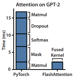
Dao et al. realized that while previous approaches aimed to reduce FLOPs, they ignored overheads from memory accesses. Semianalysis also recently pointed out that a huge chunk of the time in large model training/inference is not spent computing matrix multiplies, but rather waiting for data to get to the compute resources. This is what they called the memory wall.

FlashAttention incorporates IO awareness into the attention mechanism. It works by distributing operations between GPU memory of different speeds, which makes the entire computation process much faster. The algorithm uses tiling to reduce the number of memory reads and writes between GPU high bandwidth memory (HBM) and GPU on-chip SRAM. FlashAttention is a primitive and can be combined with block-spare attention, which makes it the quickest and most efficient approximate or non-approximate attention algorithm available today.

Background

To understand the efficiency of FlashAttention's exact attention computation, it's essential to have some knowledge about GPU memory and the performance traits of different operations on it, so let's learn about that.

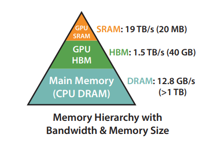
GPU Memory Hierarchy

Let's take the Nvidia A100 GPU for example. It has 40GB of High Bandwidth Memory (HBM), which despite its name is much slower than the 108 on-chip SRAM modules each 192KB in size. With time, compute has gotten much faster relative to memory speed, hence transformer-based language models are increasingly bottlenecked by memory (HBM) access rather than compute. Thus, the goal of the FlashAttention paper was to use the SRAM as well as efficiently as possible to speed up the computation.

Performance Characteristics

GPUs rely on numerous threads to simultaneously execute operations through the application of kernels. The input is loaded into the SRAM attached to the streaming multiprocessors (SMs) and their registers, and after computation eventually written back to HBM.

To better understand the bottleneck of operations let's introduce arithmetic intensity. Arithmetic intensity is a measure of floating-point operations (FLOPs) performed by a given operation relative to the number of memory accesses (Bytes) that are required to support it.

In compute-bound operations the arithmetic intensity is high. Examples of such operations are matrix multiplication with large inner dimensions and convolution with a large number of channels.

Memory-bound operations on the other hand have low arithmetic complexity and are bottlenecked by memory bandwidth. Examples are essentially all elementwise operations, e.g. activations and dropout, and reduction operations, e.g. sum, softmax, batch normalization, and layer normalization.

Following Lei Mao's great blog post, let's analyze e.g. matrix multiplication a bit more closely. With two \( N \times N \) matrices as input, we compute a new \( N \times N \) matrix as output. This requires \( 2 N^3 \) computations, \( N^3 \) multiplications and \( N^3 \) additions. With scalars encoded in \( b \) bits and without caching, the total number of bits read is \( 2bN^3 \). If we can fit one of the \(N \times N\) matrices into memory, the total number of bitwise IO operations reduces to \( 3bN^2 \). So

\[ \begin{align*} \frac{N_{\text{op}}}{N_{\text{byte}}} &= \frac{2N^3}{3bN^2 / 8} \\ &= \frac{16N}{3b} \\ &= \frac{N}{6} : \text{OP/byte} \\ \end{align*} \]

For 32-bit floats (\( b = 32 \)) and a Nvidia A100 (19.5 TFLOPS and 1.6 TB/s for FB32) we have

\[ \frac{\text{BW}_{\text{math}}}{\text{BW}_{\text{mem}}} = 12.2 : \text{OP/byte} \]

So for \( N >= 74 \) the matrix multiplication operation is compute-bound, for smaller matrix multiplications it is memory bound.

Kernel Fusion

One way to reduce the need to read from and write to HBM is the idea of kernel fusion. Here subsequent operations are fused alleviating the need to do HBM IO after each one. Note however that during model training, the efficiency of kernel fusion is often decreased due to the need to write intermediate values to the HBM for the backward pass.

Standard Attention

The standard transformer self-attention is given by

\[ Attention(Q, K, V) = softmax(\frac{QK^\mathsf{T}}{\sqrt{d_k}})V \]

Here the inputs \( Q, K, V  \in \mathbb{R}^{N \times d} \) where \( N \) is the sequence length and \( d \) is the head dimension. The attention output is \(  \in \mathbb{R}^{N \times d} \).

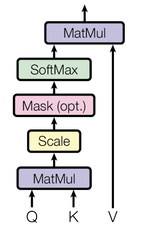
Attention is computed as

\[ \mathbf{S} = \mathbf{QK^\mathsf{T}} \in \mathbb{R}^{N \times N},\quad \mathbf{P} = softmax(\mathbf{S}) \in \mathbb{R}^{N \times N},\quad \mathbf{O} = \mathbf{PV} \in \mathbb{R}^{N \times d}  \]

The \( \mathbf{S} \) and \( \mathbf{P} \) matrices are typically so large that they need to be materialized in HBM, thus resulting in costly reads and writes. The paper introduces two improvements to the attention computation to alleviate this

1. The softmax reduction is computed without access to the whole input.
2. The large attention matrix ( \( N \times N \) is not stored for the backward pass, but rather recalculated on the fly.

This is achieved by splitting the input matrices into blocks and performing several passes over them to perform the softmax operation. The softmax normalization factor from the forward pass is stored to quickly recompute attention on-chip in the backward pass, which despite the additional divisions is faster than reading the intermediate matrix from HBM.

Overall this leads to increased FLOPS (due to recomputation), but fast wall-clock runtime and less memory use. So in a sense, the reformulation moves the operation from memory- to compute-bound.

Algorithm Deep Dive

As already mentioned, the main idea behind the algorithm is to tile the inputs \( \mathbf{Q}, \mathbf{K}, \mathbf{V} \) into blocks, load them from slow HBM to fast SRAM and compute the attention block by block. The output of each block is scaled by the appropriate normalization factor before adding them up.

Here is the algorithm description from the paper. Let's go through it step by step

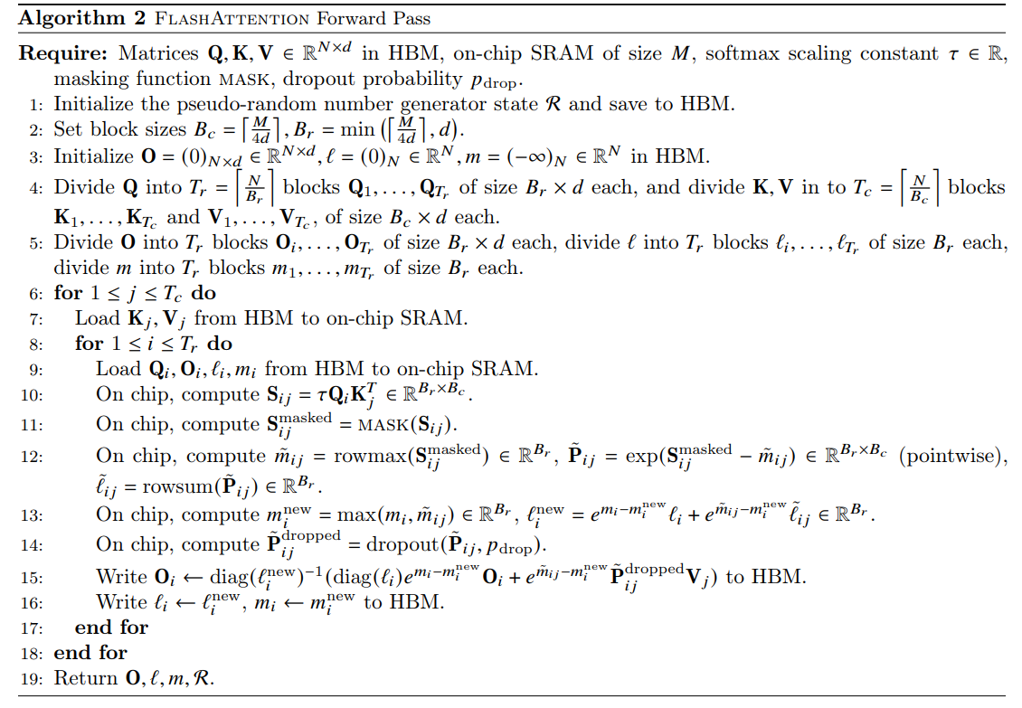
Tiling

The key part to understanding is the block-wise computation of the softmax. he softmax of a vector \( x \) can be computed as

\[ m(x) = \max_i x_i,\; f(x) = \left[ e^{x_1 - m(x)} ... e^{x_B - m(x)}  \right], \; l(x) = \sum_i f(x_i), \; \textrm{softmax}= \frac{f(x)}{l(x)} \]

If we split the vector \( x \) into \( x^{(1)} \) and \(  x^{(2)} \) with \( x = \left[ x^{(1)} x^{(2)} \right] \in \mathbb{R}^{2B} \), we can perform above calculation in two steps.

1. Perform above calculation for \( x^{(1)} \) and \(  x^{(2)} \) respectively.
2. Combine the results by rescaling \( l( x^{(1)} ) \) and \( l( x^{(2)} ) \) appropriately.

Specifically,

\[ m(x) = \max(m(x^{(1)}), m(x^{(2)})), \; l(x) = e^{m(x^{(1)}) - m(x)} l(x^{(1)}) + e^{m(x^{(2)}) - m(x)} l(x^{(2)}) \]

Recomputation

The backward pass of FlashAttention requires the \( \mathbf{S} \) and \( \mathbf{P} \) matrices to compute the gradients w.r.t. \( \mathbf{Q} \) , \( \mathbf{K} \) and \( \mathbf{V} \). These are large \( N \times N \) matrices and would surely not fit into SRAM requiring a costly HBM lookup. The trick is to perform a blockwise reconstruction of \( \mathbf{S} \) and \( \mathbf{P} \) from blocks of \( \mathbf{Q} \) , \( \mathbf{K} \) and \( \mathbf{V} \) in SRAM using the statistics \( l(x) \) and \( m(x) \).

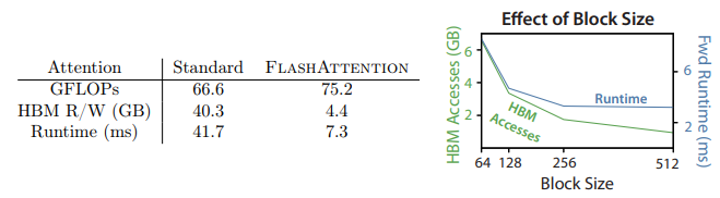
IO Complexity of FlashAttention

The authors show that for a sequence of length \( N \), head dimension \( d \) and SRAM of size \( M \), standard attention requires \( \mathcal{O}(N d + N^2)  \) HBM accesses, while FlashAttention requires  \( \mathcal{O}(N^2 d^2 M^{-1} )  \) HBM accesses.

For typical values of \( d \) (64 - 128) and M (around 100KB), \( d^2 \) is many times smaller than \( M \), and thus FlashAttention requires fewer HBM accesses.

Source Code

You can find both a CUDA and OpenAI Triton implementation on Github here

GitHub - HazyResearch/flash-attention: Fast and memory-efficient exact attention

Fast and memory-efficient exact attention. Contribute to HazyResearch/flash-attention development by creating an account on GitHub.

GitHubHazyResearch